Computing Quadratures of Polynomial Functions over k-Simplices \(\triangle^k\) in \(\mathbb{R}^n\)

Contents:

Suppose we are given a k-Simplex \(\triangle^k\) in \(\mathbb{R}^n\)

\[\triangle^k=\left\{ \sum_{i=0}^{k}\lambda_{i}\mathbf{x}_{i}\vert\lambda_{i}\ge0,\,0\leq i\le k,\,\sum_{i=0}^{k}\lambda_{i}=1\right\}\]

where \(\mathbf{x}_i\) represents the i^th vertex of the simplex.

\[\begin{split}\mathbf{x}_{1}=\left(\begin{array}{c} x_{1}\\ y_{1}\\ z_{1}\\ \vdots \end{array}\right)\qquad\mathbf{x}_{2}=\left(\begin{array}{c} x_{2}\\ y_{2}\\ z_{2}\\ \vdots \end{array}\right)\dots\qquad\mathbf{x}_{i}=\left(\begin{array}{c} x_{i}\\ y_{i}\\ z_{i}\\ \vdots \end{array}\right)\dots\qquad\mathbf{x}_{k}=\left(\begin{array}{c} x_{k}\\ y_{k}\\ z_{k}\\ \vdots \end{array}\right)\end{split}\]

We are interested in finding an explicit expression for the quadrature of a homogeneous polynomial over such a simplex:

\[\int_{\triangle_{k}}x^{\alpha}y^{\beta}\dots\]

and the moments, which are the above expression divided by the volume of the simplex:

\[\langle x^\alpha y^\beta \dots \rangle = \frac{1}{\text{vol} (\triangle_k)} \int_{\triangle_{k}}x^{\alpha}y^{\beta}\dots\]

We have implemented in python a simple algorithm that computes exactly the above expressions:

quadrature.nCk(n, k)

Compute the binomial coefficients \(\binom nk = \frac{n!}{k!(n-k)!}\)

>>> nCk(0,0)
1
>>> nCk(1,0)
1
>>> nCk(4, 2)
6
>>> [[nCk(n,k) for k in range(n+1)] for n in range(7)] == [
...          [1],
...        [1, 1],
...       [1, 2, 1],
...      [1, 3, 3, 1],
...     [1, 4, 6, 4, 1],
...    [1, 5, 10, 10, 5, 1],
...  [1, 6, 15, 20, 15, 6, 1]                              ]
True

quadrature.quadrature(term, verts)

Compute the quadrature of a homogenous polynomial given by term=’xxy’ over the vertices verts=(0,1,2) of a simplex.

>>> quadrature('', (0,1))
([((), 1)], Fraction(1, 1))
>>> quadrature('x', (0,1))
([((('x', 0),), 1), ((('x', 1),), 1)], Fraction(1, 2))
>>> quadrature('x', (0,1,2))
([((('x', 0),), 1), ((('x', 1),), 1), ((('x', 2),), 1)], Fraction(1, 3))
>>> quadrature('xx', (0,1)) == (
...    [((('x', 0), ('x', 0)), 1),
...     ((('x', 0), ('x', 1)), 1),
...     ((('x', 1), ('x', 1)), 1)], fractions.Fraction(1, 3))
True
>>> quadrature('xy', (0,1,2)) == (
...    [((('x', 0), ('y', 0)), 2),
...      ((('x', 0), ('y', 1)), 1),
...      ((('x', 0), ('y', 2)), 1),
...      ((('x', 1), ('y', 0)), 1),
...      ((('x', 1), ('y', 1)), 2),
...      ((('x', 1), ('y', 2)), 1),
...      ((('x', 2), ('y', 0)), 1),
...      ((('x', 2), ('y', 1)), 1),
...      ((('x', 2), ('y', 2)), 2)], fractions.Fraction(1, 12))
True

Description of Algorithm

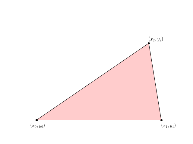
Our algorithm is general, but for simplicity we will just demonstrate it for the specific case of a triangle in two dimensions. Assume you have a triangle in the plane defined by its three vertices at \((x_0,y_0)\), \((x_1,y_1)\), and \((x_2,y_2)\) - it is a 2-simplex so \(k=2\). We will compute the moment of the q-homoqenous polynomial \(\langle xy \rangle\) with \(q=2\).

(Source code, png, hires.png, pdf)

The inputs to the algorithm are two tuples - the first is \(\text{term}=(x,y)\) describing the polynomial and the other is \(\text{verts}=(0,1,2)\) describing the labels for the vertices. With this notation, the orders of the simplex \(k\) and the degree of the polynomial \(q\) are given by

\[\begin{split}k &= \text{len}(\text{verts})-1 = 2 \\ q &= \text{len}(\text{term}) = 2\\\end{split}\]

Now take all the permutations of the \(\text{term}\) tuple.

\[P = \mathcal{P}(\text{term}) = (xy, yx)\]

Compute all the combinations (with repetitions allowed) of size \(q=2\) of the coordinates of the vertices

\[V = \mathcal{C}^q(\text{verts}) = (00, 01, 02, 11, 12, 22)\]

Take the product of \(V\) and \(P\)

\[P \times V = \left ( (xy,00), (xy,01),(xy,02),(xy,11),(xy,12),(xy,22), (yx,00),(yx,01),(yx,02),(yx,11),(yx,12),(yx,22) \right)\]

For each element in the tuple zip together the variable with the simplex vertices (e.g. \((xy,00) \mapsto x_0y_0, \quad (xy,01) \mapsto x_0y_1\) and so on):

\[\text{zip}(P \times V) = \left ( x_0 y_0, x_0 y_1, x_0 y_2, x_1 y_1, x_1y_2, x_2y_2, y_0x_0, y_0x_1,y_0x_2,y_1x_1,y_1x_2,y_2x_2 \right)\]

Treat each element as a multiplication and sum all the multiples together

\[\sum(\text{zip}(P \times V)) = \left ( 2 x_0 y_0 + x_0 y_1 + x_0 y_2 + x_1 y_0 + 2 x_1 y_1 + x_1 y_2 + x_2 y_0 + x_2 y_1 + 2 x_2 y_2 \right)\]

Divide the result by \(\binom{k+q}{q} q!\) to obtain the final expression

\[\frac{1}{\binom{k+q}{q} q!} \sum(\text{zip}(P \times V)) = \frac{1}{12} \left ( 2 x_0 y_0 + x_0 y_1 + x_0 y_2 + x_1 y_0 + 2 x_1 y_1 + x_1 y_2 + x_2 y_0 + x_2 y_1 + 2 x_2 y_2 \right)\]

which is indeed what one would obtain for \(\langle xy \rangle\) by manual calculation.

Pseudocode

In pseudocode the algorithm can be concisely given as:

\[\begin{split}& \text{def quadrature}(\text{term},\,\text{verts}): \\ & \qquad k = \text{len}(\text{verts})-1 \\ & \qquad q = \text{len}(\text{term}) \\ & \qquad P = \mathcal{P}(\text{term}) \\ & \qquad V = \mathcal{C}^q(\text{verts}) \\ & \qquad \text{return} \quad \frac{1}{\binom{k+q}{q} q!} \sum(\text{zip}(P \times V))\end{split}\]

Validation

To validate the algorithm we consider a triangle, a line segment, and a tetrahedron, and we compute a number of low order moments by integrating explicitly. The Mathematica file where all the integration is done is provided for download here.

Triangle \(\triangle^2\) in \(\mathbb{R}^2\)

The moments of all the homogeneous polynomials over a triangle area given by

\[\langle x^{n}y^{m}\rangle=\frac{1}{A}\int_{\triangle}x^{n}y^{m}\,\mathbf{d}x\wedge\mathbf{d}y\]

where \(\mathbf{d}x\wedge\mathbf{d}y\) is the area form for \(\mathbb{R}^2\) and \(A=\int_{\triangle}\mathbf{d}x\wedge\mathbf{d}y\) is the total area of the triangle.

For example, \(\langle x \rangle\) and \(\langle y \rangle\) are the coordinates of the center of mass of the triangle.

Change of variables \(x,y \mapsto s,t\)

\[\begin{split}x &= (1-s-t)x_{0}+sx_{1}+tx_{2}=s(x_{1}-x_{0})+t(x_{2}-x_{0}) \\ y &= (1-s-t)y_{0}+sy_{1}+ty_{2}=s(y_{1}-y_{0})+t(y_{2}-y_{0})\end{split}\]

so that \((s,t)=(0,0)\) corresponds to vertex \((x_{0},y_{0})\), \((s,t)=(1,0)\) corresponds to vertex \((x_{1},y_{1})\), and \((s,t)=(0,1)\) corresponds to vertex \((x_{2},y_{2})\). The area form transforms as follows:

\[\begin{split}dx\wedge dy &= \left((x_{1}-x_{0})(y_{2}-y_{0})-(x_{2}-x_{0})(y_{1}-y_{0})\right)\, ds\wedge dt \\ &= 2A\, ds\wedge dt\end{split}\]

Thus we have an explicit expression for the quadrature

\[\langle x^{n}y^{m}\rangle=2\int_{0}^{1}ds\int_{0}^{1-s}dt\left(s(x_{1}-x_{0})+t(x_{2}-x_{0})\right)^{n}\left(s(y_{1}-y_{0})+t(y_{2}-y_{0})\right)^{m}dt\]

which can be evaluated by hand to obtain the first few moments:

\[\begin{split}\frac{1}{6} \left(x_{0}^{2} + x_{0} x_{1} + x_{0} x_{2} + x_{1}^{2} + x_{1} x_{2} + x_{2}^{2}\right) \\ \frac{1}{10} \left(x_{0}^{3} + x_{0}^{2} x_{1} + x_{0}^{2} x_{2} + x_{0} x_{1}^{2} + x_{0} x_{1} x_{2} + x_{0} x_{2}^{2} + x_{1}^{3} + x_{1}^{2} x_{2} + x_{1} x_{2}^{2} + x_{2}^{3}\right) \\ \frac{1}{12} \left(2 x_{0} y_{0} + x_{0} y_{1} + x_{0} y_{2} + x_{1} y_{0} + 2 x_{1} y_{1} + x_{1} y_{2} + x_{2} y_{0} + x_{2} y_{1} + 2 x_{2} y_{2}\right) \\ \frac{1}{21} \left(x_{0}^{5} + x_{0}^{4} x_{1} + x_{0}^{4} x_{2} + x_{0}^{3} x_{1}^{2} + x_{0}^{3} x_{1} x_{2} + x_{0}^{3} x_{2}^{2} + x_{0}^{2} x_{1}^{3} + x_{0}^{2} x_{1}^{2} x_{2} + x_{0}^{2} x_{1} x_{2}^{2} + x_{0}^{2} x_{2}^{3} + x_{0} x_{1}^{4} + x_{0} x_{1}^{3} x_{2} + x_{0} x_{1}^{2} x_{2}^{2} + x_{0} x_{1} x_{2}^{3} + x_{0} x_{2}^{4} + x_{1}^{5} + x_{1}^{4} x_{2} + x_{1}^{3} x_{2}^{2} + x_{1}^{2} x_{2}^{3} + x_{1} x_{2}^{4} + x_{2}^{5}\right) \\\end{split}\]

\[\begin{split}\langle 1 \rangle &= 1 \\ \langle x \rangle &= \frac{1}{3}( x_0 + x_1 + x_2 ) \\ \langle x^2 \rangle &= \frac{1}{6}( x_0^2 + x_0 x_1 + x_1^2 + x_0 x_2 + x_1 x_2 + x_2^2 ) \\ \langle x^3 \rangle &= \frac{1}{10}( x_0^3 + x_0^2 x_1 + x_0 x_1^2 + x_1^3 + x_0^2 x_2 + x_0 x_1 x_2 + x_1^2 x_2 + x_0 x_2^2 + x_1 x_2^2 + x_2^3 ) \\ \langle x y \rangle &= \frac{1}{12}( 2 x_0 y_0 + x_1 y_0 + x_2 y_0 + x_0 y_1 + 2 x_1 y_1 + x_2 y_1 + x_0 y_2 + x_1 y_2 + 2 x_2 y_2 ) \\\end{split}\]

Those match exactly with the results from our algorithm.

quadrature.test_triangle()

>>> def q(t): return tostr(quadrature(t, (0,1,2)))
>>> q('x')
'1/3 (x0 + x1 + x2)'
>>> q('xx')
'1/6 (x0x0 + x0x1 + x0x2 + x1x1 + x1x2 + x2x2)'
>>> q('xxx')
'1/10 (x0x0x0 + x0x0x1 + x0x0x2 + x0x1x1 + x0x1x2 + x0x2x2 + x1x1x1 + x1x1x2 + x1x2x2 + x2x2x2)'
>>> q('xy')
'1/12 (2 x0y0 + x0y1 + x0y2 + x1y0 + 2 x1y1 + x1y2 + x2y0 + x2y1 + 2 x2y2)'

Line Segment \(\triangle^1\) in \(\mathbb{R}^2\)

The same be done for line segments defined by their endpoints \((x_0,y_0)\) and \((x_1,y_1)\). Again the first few moments in this case are:

\[\begin{split}\langle 1 \rangle &= 1 \\ \langle x \rangle &= \frac{1}{2}(x_0 + x_1) \\ \langle x^2 \rangle &= \frac{1}{3}(x_0^2 + x_0 x1 + x_1^2) \\ \langle x^3 \rangle &= \frac{1}{4}(x_0^3 + x_0^2 x_1 + x_0 x_1^2 + x_1^3) \\ \langle x y \rangle &= \frac{1}{6}(2 x_0 y_0 + x_1 y_0 + x_0 y_1 + 2 x_1 y_1) \\ \langle x^2 y \rangle &= \frac{1}{12}(3 x_0^2 y_0 + 2 x_0 x_1 y_0 + x_1^2 y_0 + x_0^2 y_1 + 2 x_0 x_1 y_1 + 3 x_1^2 y_1) \\\end{split}\]

And our algorithm gives

quadrature.test_line_segment()

>>> def q(t): return tostr(quadrature(t, (0,1)))
>>> q('x')
'1/2 (x0 + x1)'
>>> q('xx')
'1/3 (x0x0 + x0x1 + x1x1)'
>>> q('xxx')
'1/4 (x0x0x0 + x0x0x1 + x0x1x1 + x1x1x1)'
>>> q('xy')
'1/6 (2 x0y0 + x0y1 + x1y0 + 2 x1y1)'
>>> q('xxy')
'1/12 (3 x0x0y0 + x0x0y1 + 2 x0x1y0 + 2 x0x1y1 + x1x1y0 + 3 x1x1y1)'

Tetrahedron \(\triangle^3\) in \(\mathbb{R}^3\)

\[\begin{split}\langle 1 \rangle &= 1 \\ \langle x \rangle &= \frac{1}{4}(x_0 + x_1 + x_2 + x_3) \\ \langle x^2 \rangle &= \frac{1}{20}(2 x_0^2 + 2 x_0 x_1 + 2 x_1^2 + 2 x_0 x_2 + 2 x_1 x_2 + 2 x_2^2 + 2 x_0 x_3 + 2 x_1 x_3 + 2 x_2 x_3 + 2 x_3^2) \\ \langle x^3 \rangle &= \frac{1}{20}(x_0^3 + x_0^2 x_1 + x_0 x_1^2 + x_1^3 + x_0^2 x_2 + x_0 x_1 x_2 + x_1^2 x_2 + x_0 x_2^2 + x_1 x_2^2 + x_2^3 + x_0^2 x_3 + x_0 x_1 x_3 + x_1^2 x_3 + x_0 x_2 x_3 + \\ & + x_1 x_2 x_3 + x_2^2 x_3 + x_0 x_3^2 + x_1 x_3^2 + x_2 x_3^2 + x_3^3) \\ \langle xy \rangle &= \frac{1}{20}(2 x_0 y_0 + x_1 y_0 + x_2 y_0 + x_3 y_0 + x_0 y_1 + 2 x_1 y_1 + x_2 y_1 + x_3 y_1 + x_0 y_2 + x_1 y_2 + 2 x_2 y_2 + x_3 y_2 + x_0 y_3 + x_1 y_3 + x_2 y_3 + 2 x_3 y_3) \\\end{split}\]

quadrature.test_tetrahedron()

>>> def q(t): return tostr(quadrature(t, (0,1,2,3)))
>>> q('x')
'1/4 (x0 + x1 + x2 + x3)'
>>> q('xx')
'1/10 (x0x0 + x0x1 + x0x2 + x0x3 + x1x1 + x1x2 + x1x3 + x2x2 + x2x3 + x3x3)'
>>> q('xxx')
'1/20 (x0x0x0 + x0x0x1 + x0x0x2 + x0x0x3 + x0x1x1 + x0x1x2 + x0x1x3 + x0x2x2 + x0x2x3 + x0x3x3 + x1x1x1 + x1x1x2 + x1x1x3 + x1x2x2 + x1x2x3 + x1x3x3 + x2x2x2 + x2x2x3 + x2x3x3 + x3x3x3)'
>>> q('xy')
'1/20 (2 x0y0 + x0y1 + x0y2 + x0y3 + x1y0 + 2 x1y1 + x1y2 + x1y3 + x2y0 + x2y1 + 2 x2y2 + x2y3 + x3y0 + x3y1 + x3y2 + 2 x3y3)'

Indices and tables

• Index
• Module Index
• Search Page