The chain collocation method: A spectrally accurate calculus of forms
The figures below were used in the paper published here.
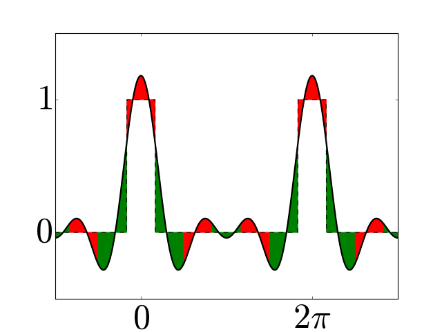
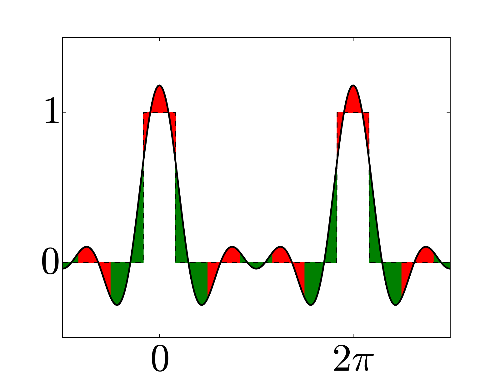
Figure 3
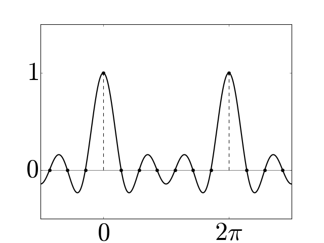
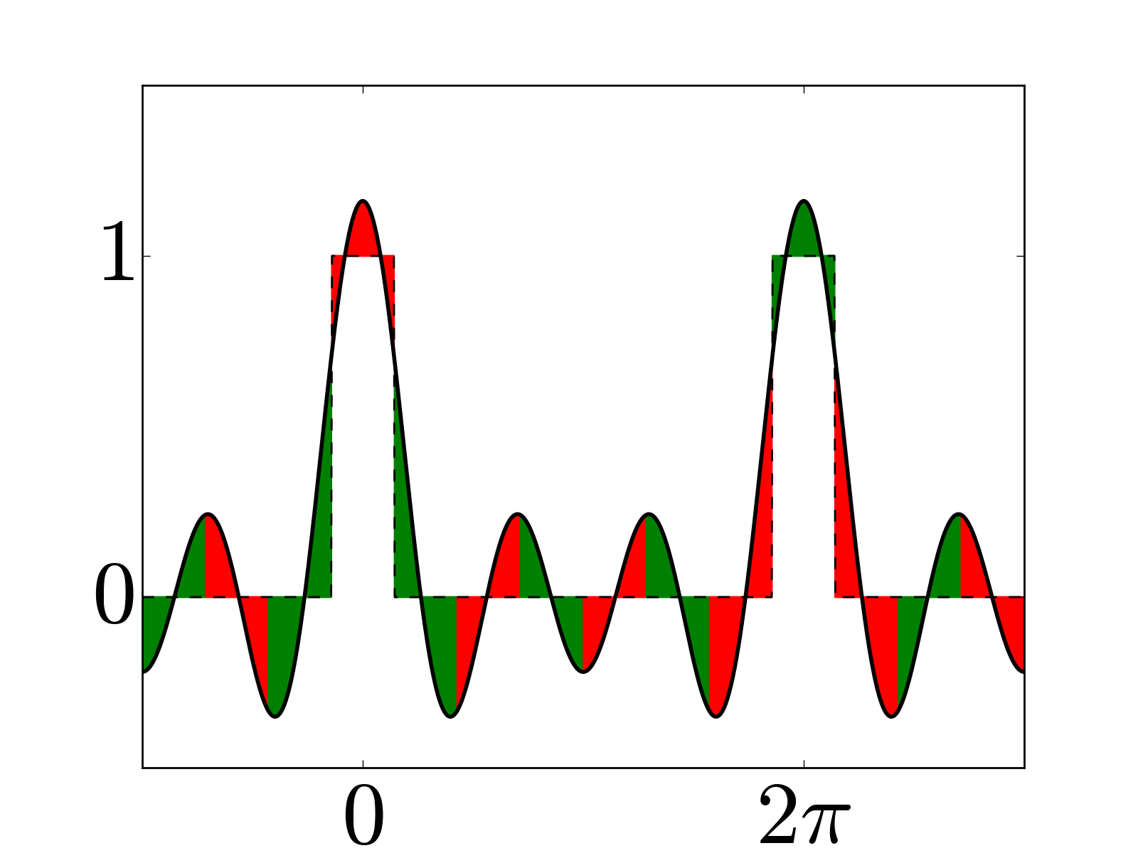
Examples of periodic interpolators for \(N=6\) (a) and \(7\) (b), and corresponding periodic histopolators (c) and (d), scaled by \(h=2\pi/N\) for clarity. While the interpolator \(\alpha_N\) satisfies \(\alpha_N(nh \mod 2\pi) = \delta_{0n} \; \forall n\), the histopolator \(\beta_N\) integrates to \(1\) over the dual cell straddling \(x=0\), and to \(0\) over other dual cells in the range \([0,2\pi]\). Note that the alternating red and green colors are used to mark out dual cells, and to illustrate that the integral of \(\beta_N\) over each of these dual cells sums to zero or one.


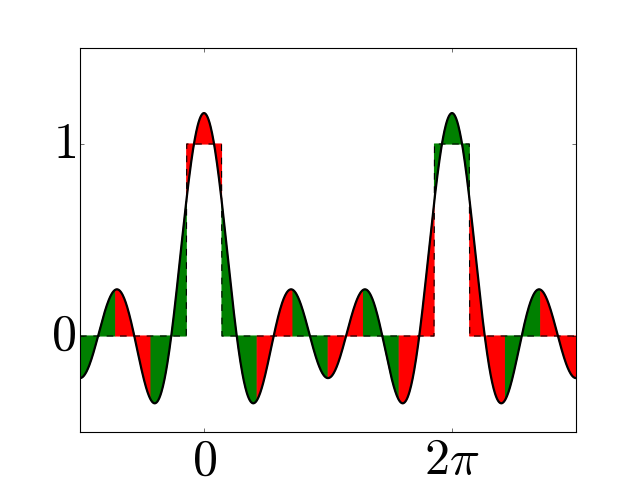
Figure 5
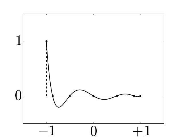
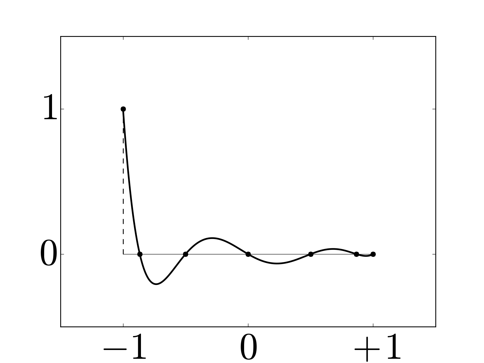
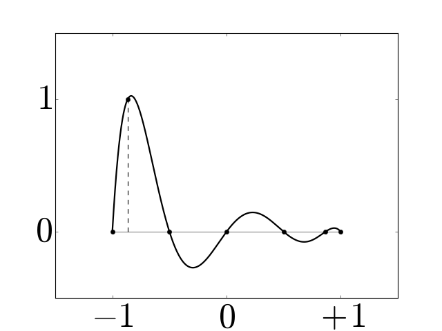
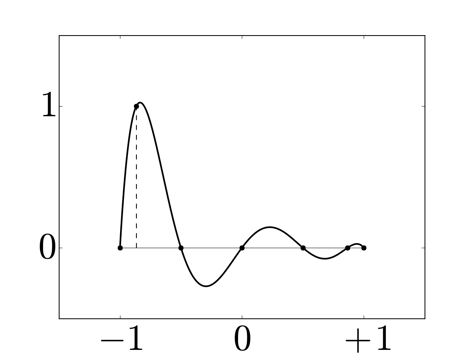
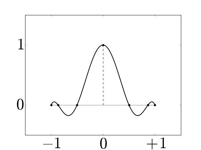
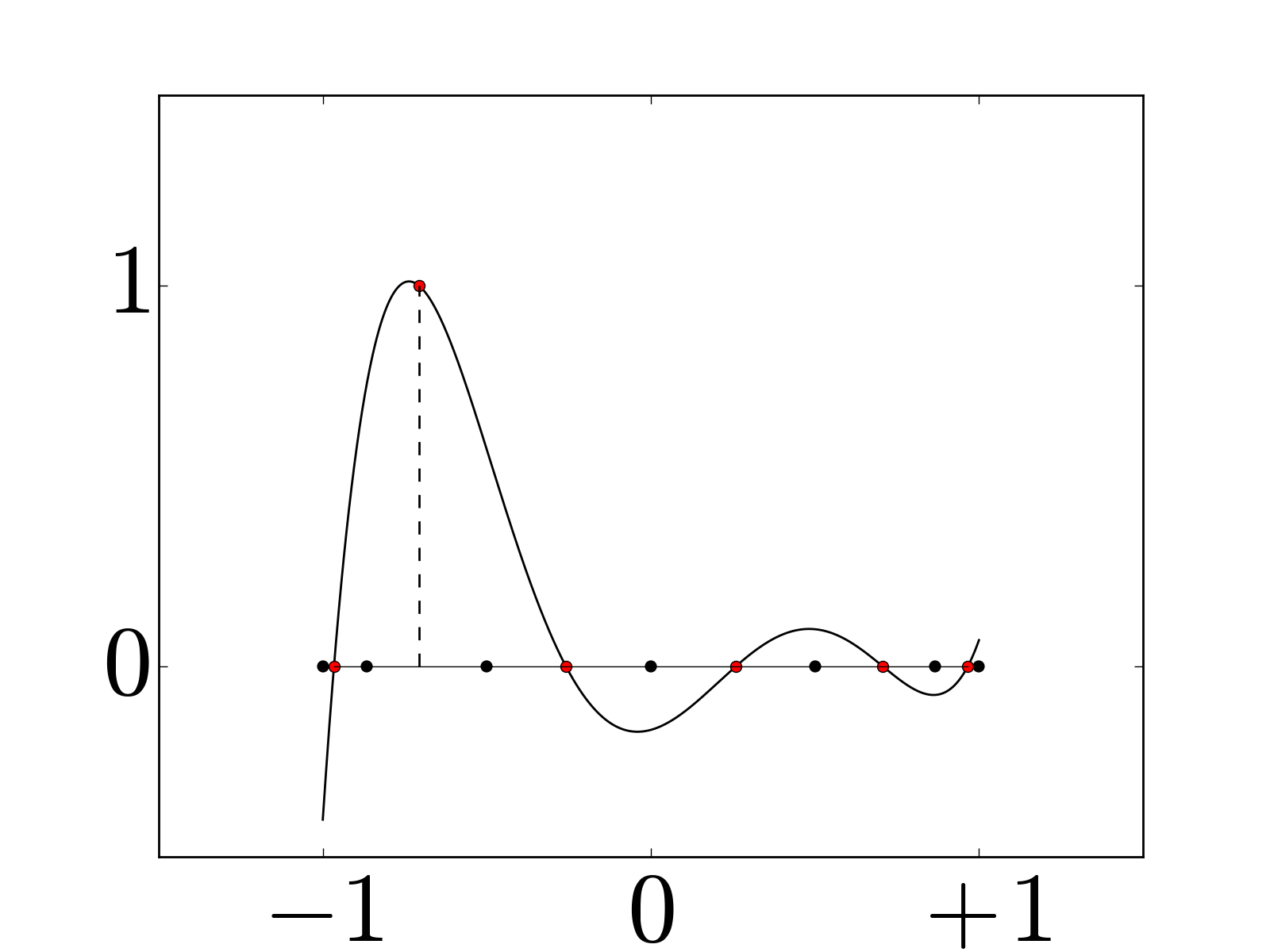
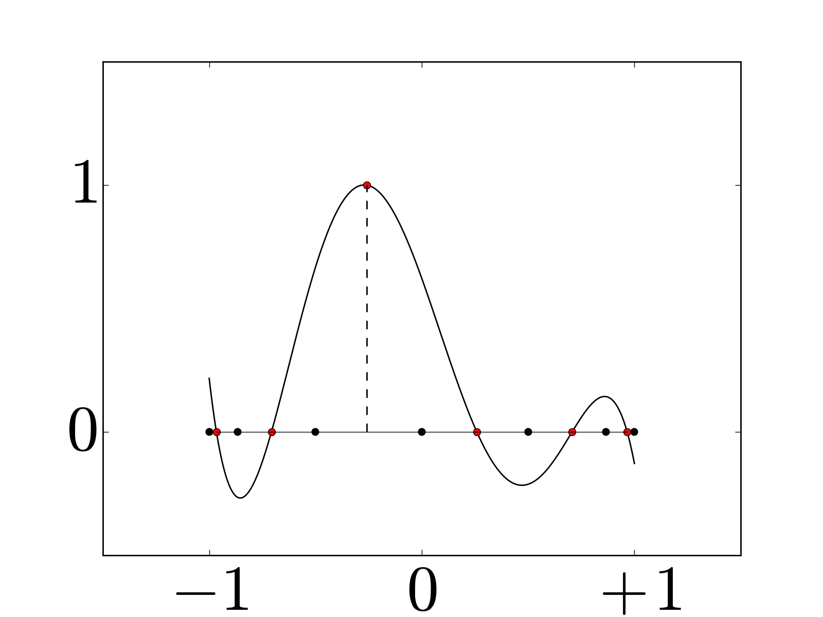
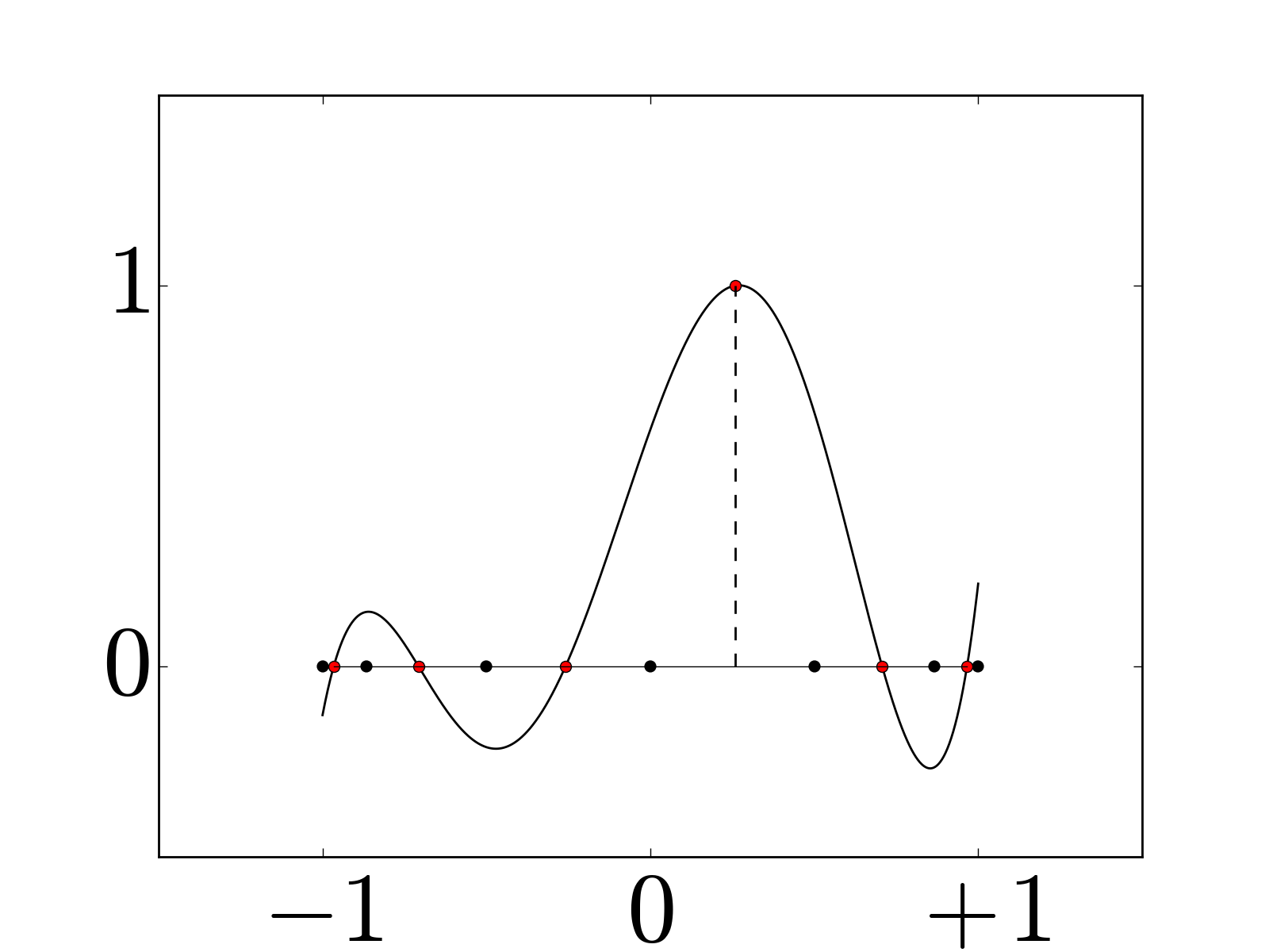
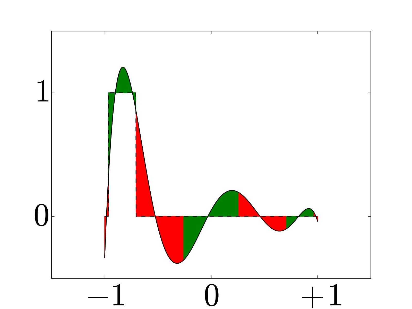
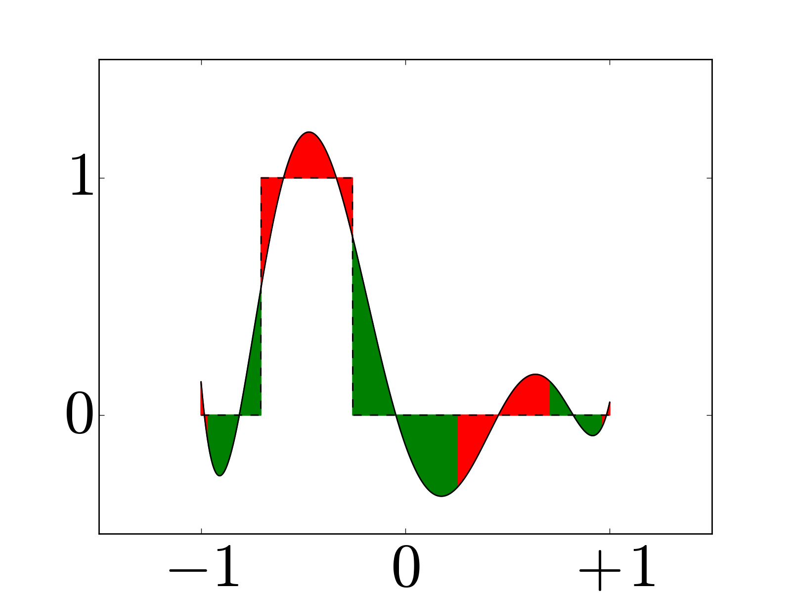
Chebyshev primal basis functions for a grid with \(N=7\). We normalize the one-form basis functions by \(x_n\!-\!x_{n-1}\) to have approximately the same scale in our visualizations.


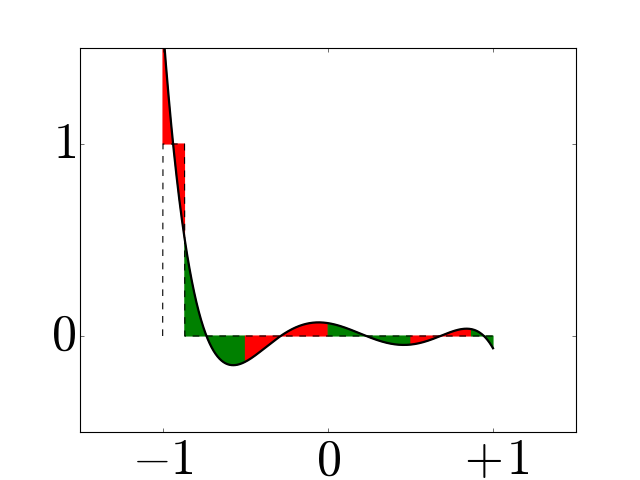
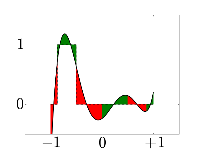
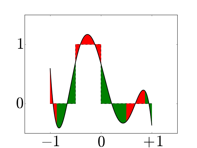
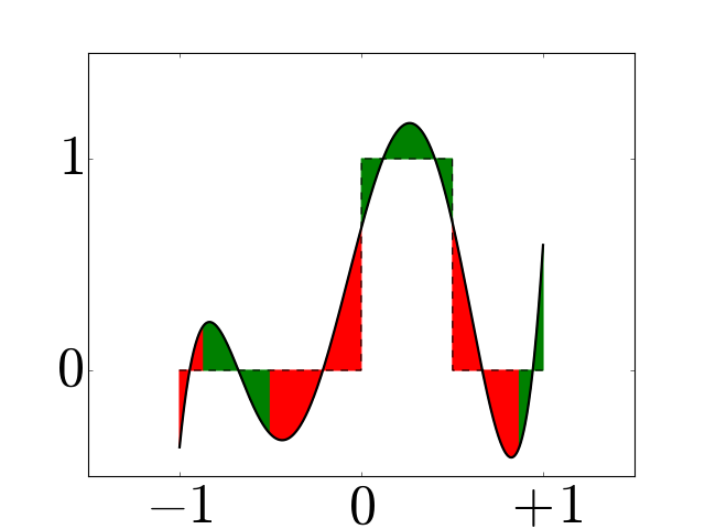
Figure 6
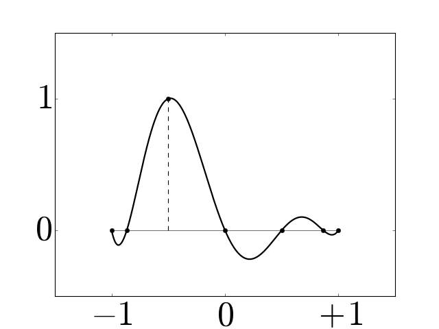
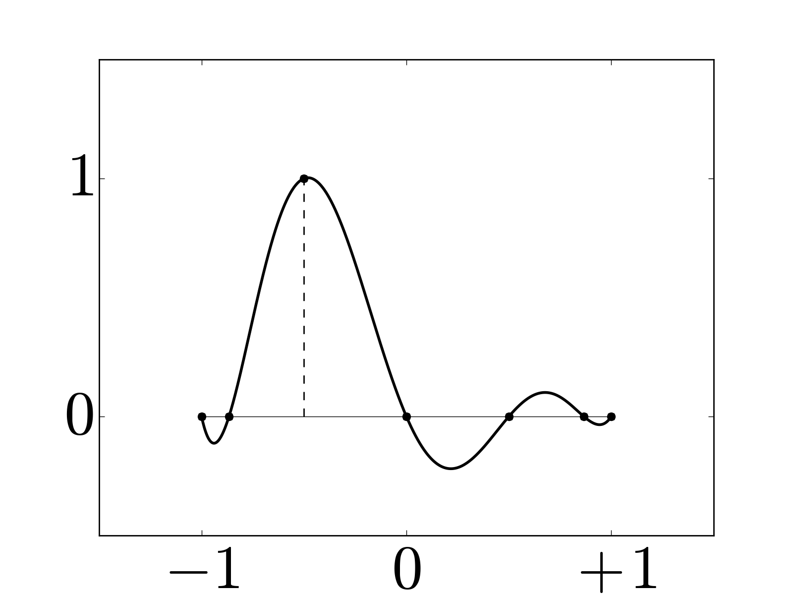
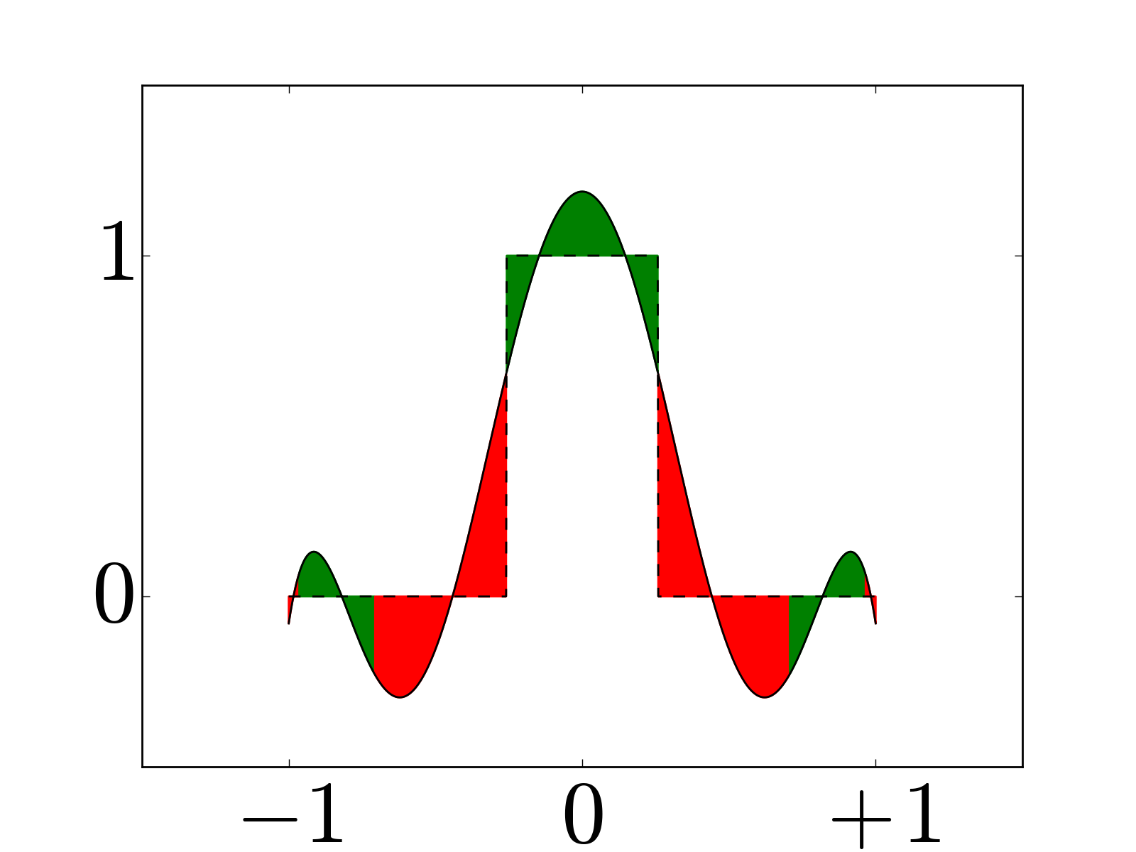
Chebyshev dual basis functions for a grid with \(N=7\).
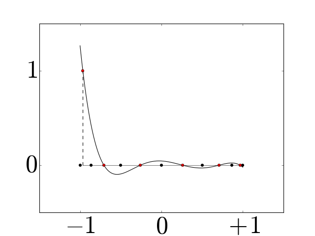
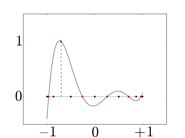

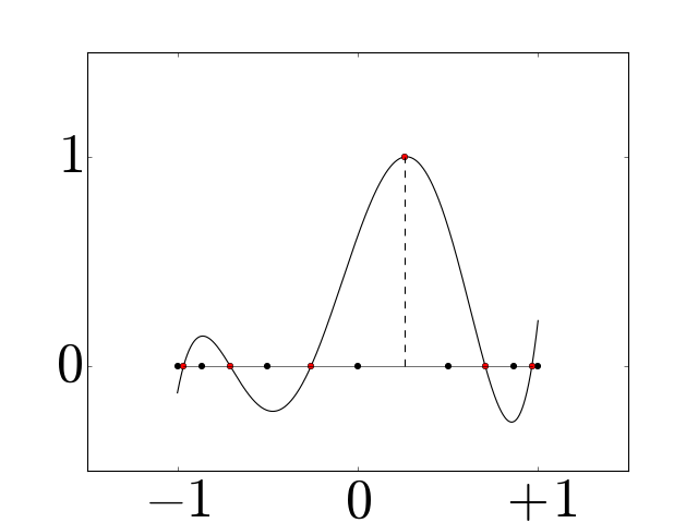
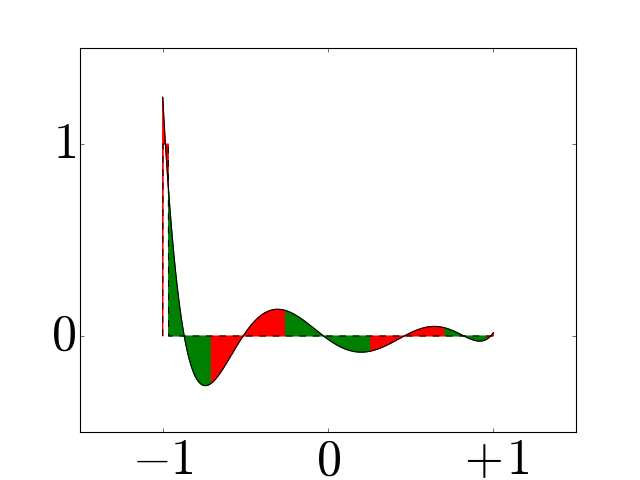


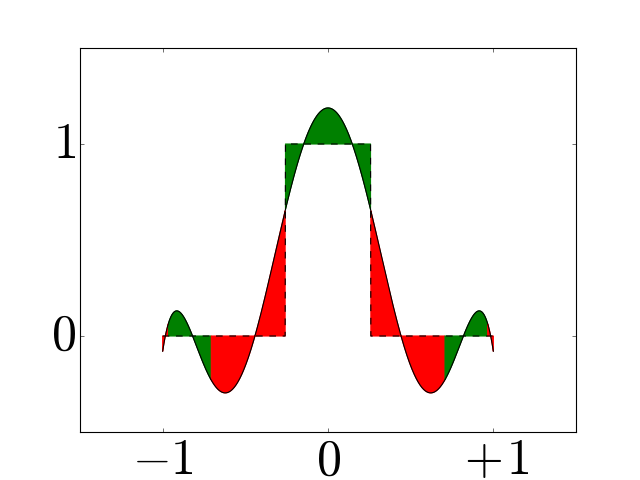
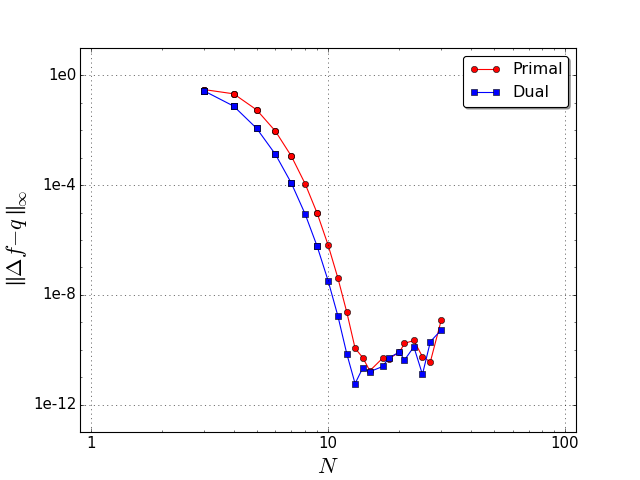
Figure 7
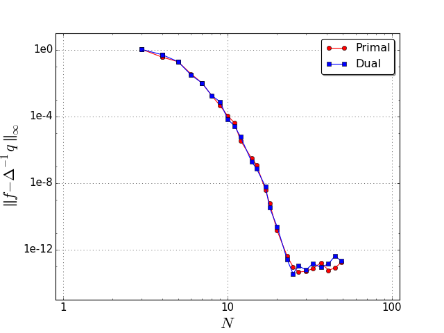
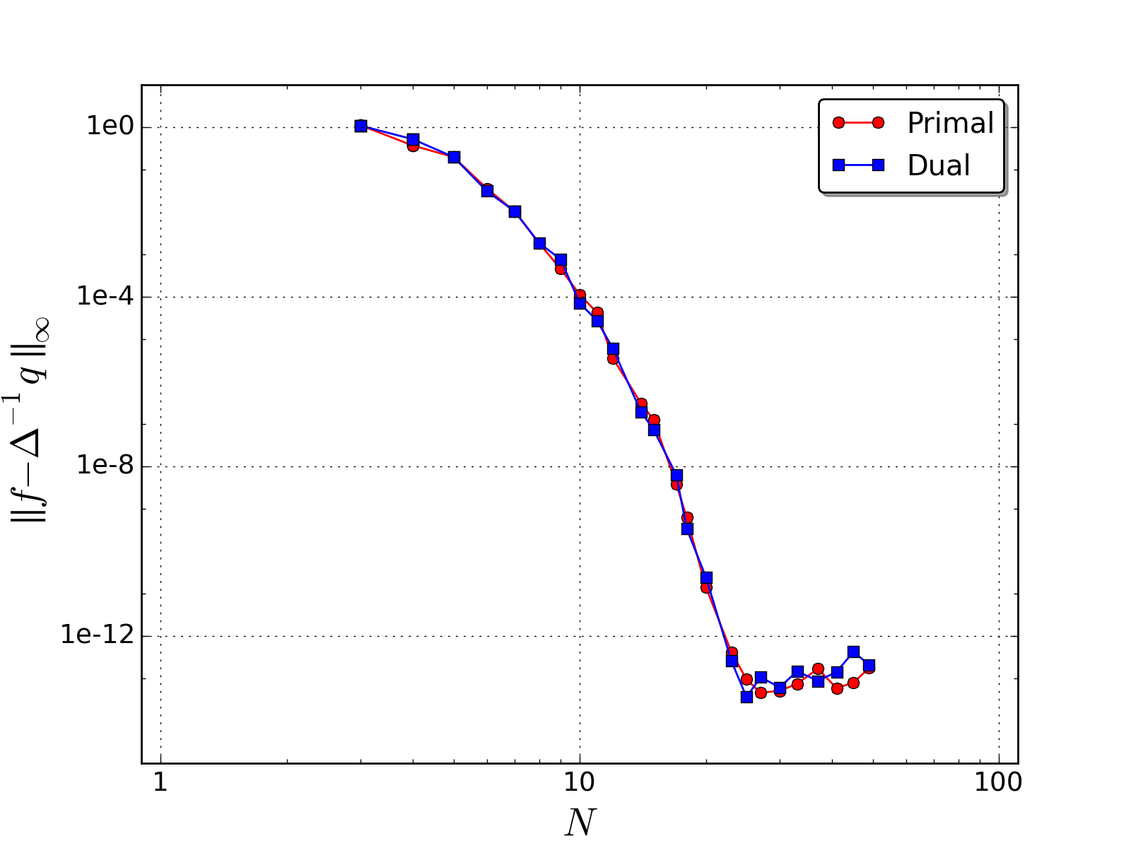
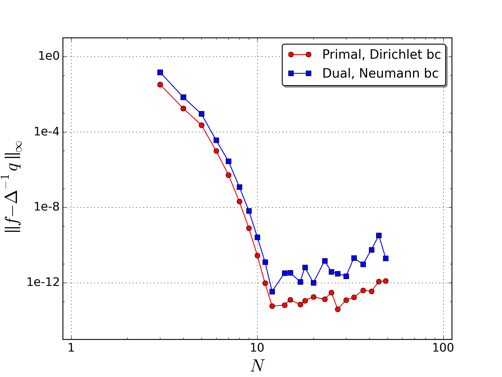
Convergence graphs for a 1D Poisson equation: (a) we solve \(\Delta f = e^{\sin x} (\cos^2 x - \sin x)\) on a periodic domain for either a primal, or dual \(0\)-form \(f\); (b) we solve math:Delta f = e^{x} on a Chebyshev grid, for either a primal \(0\)-form with Dirichlet boundary conditions \(f(-1)=e^{-1}\) and \(f(1)=e\), or for a dual \(0\)-form with Neumann boundary conditions math:f^prime(-1)= e^{-1} and \(f^\prime(+1)= e\). All of our results exhibit spectral convergence (measured through the \(L^\infty\) error \(\|f - \Delta^{-1}q \|_\infty\)), with the conventional plateau when we reach the limit of accuracy of the representation of floating point numbers.
(Source code, png, hires.png, pdf)
(Source code, png, hires.png, pdf)
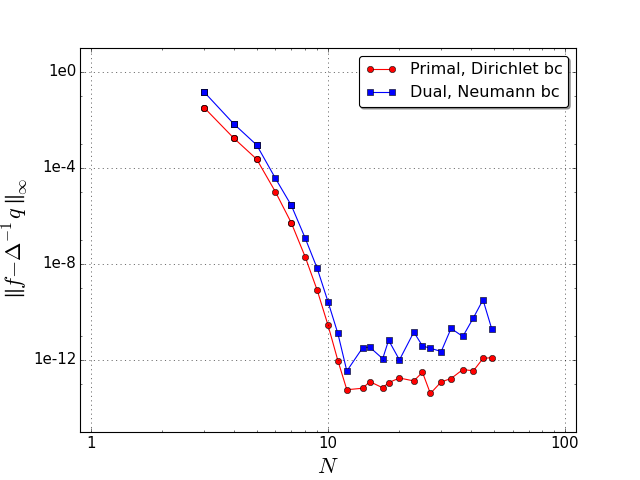
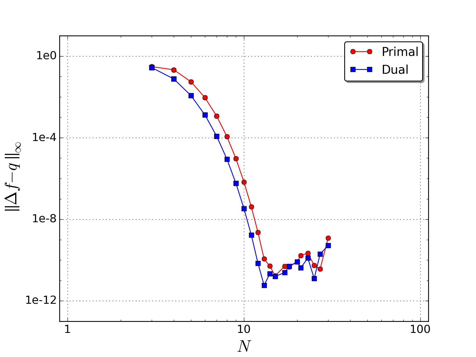
Figure 8
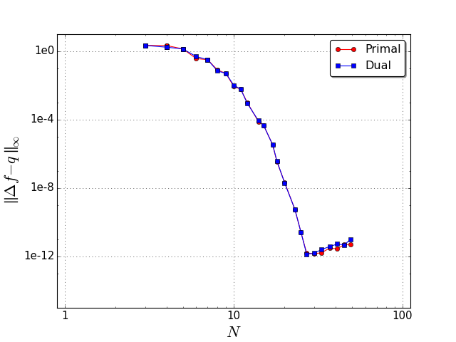
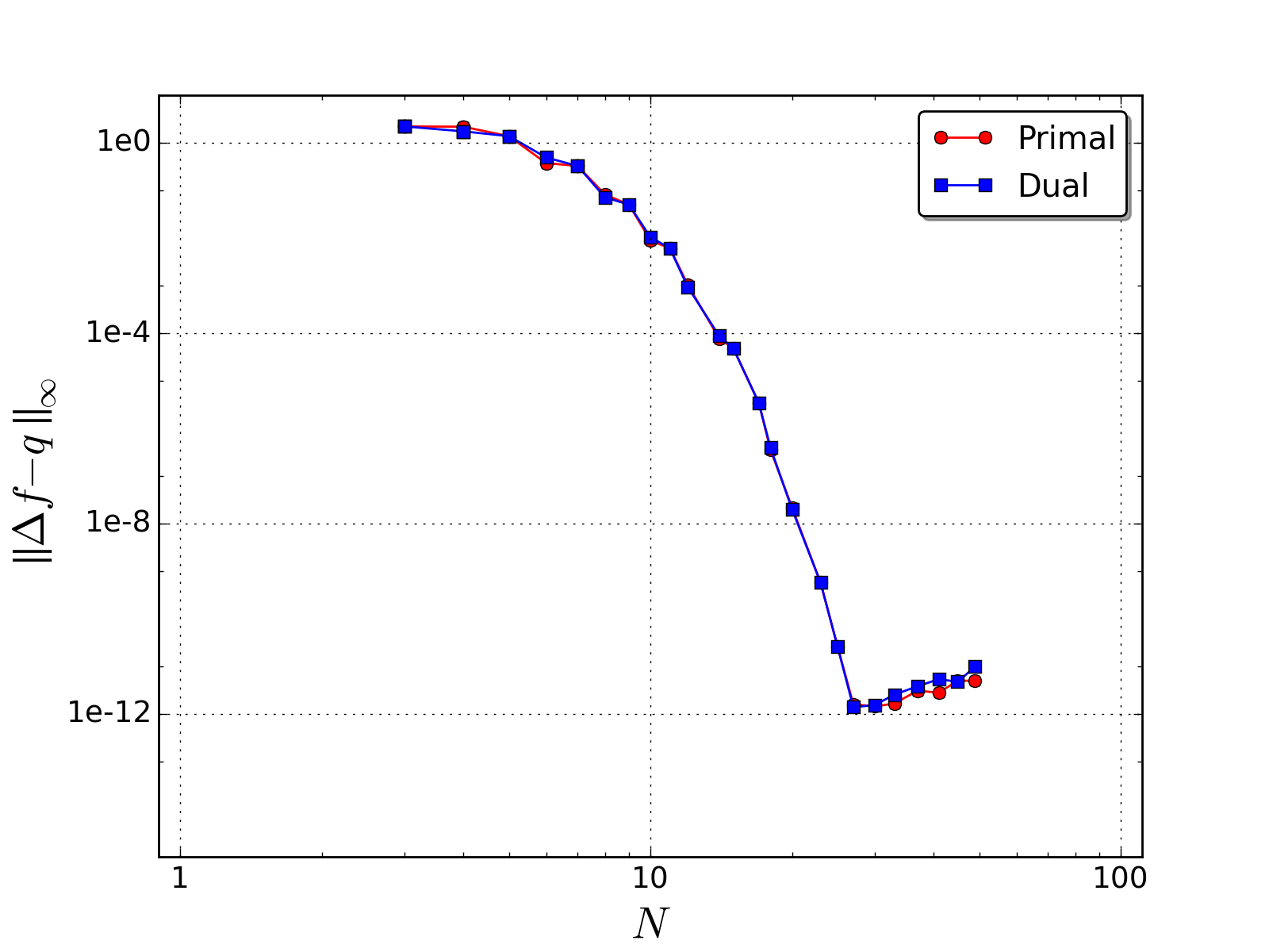
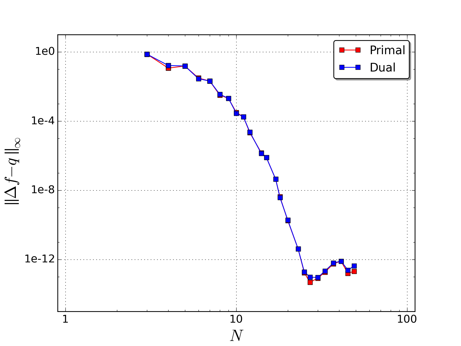
Convergence graphs for a 2D Poisson equation; (a) we solve \(\Delta f = e^{\sin x} (\cos^2 x - \sin x)+e^{\sin y} (\cos^2 y - \sin y)\) on a periodic domain for either a primal, or dual \(0\)-form \(f\); (b) Now for \(\Delta f = e^{\sin x} (\cos^2 x - \sin x) \mathbf{d}x +e^{\sin y} (\cos^2 y - \sin y) \mathbf{d}y\); (c) we solve \(\Delta f = e^{x}+e^{y}\) on a Chebyshev grid, for either a primal \(0\)-form with Dirichlet boundary conditions \(f(x,y)=e^{x}+e^{y}\), or for a dual \(0\)-form with Neumann boundary conditions \(\nabla f(x) \cdot \mathbf{n} = (e^x\;e^y)^t \;\mathbf{n}\); (d) Now for \(\Delta f = e^{x} \mathbf{d}x+e^{y}\mathbf{d}y\). All of our results exhibit spectral convergence (measured through the \(L^\infty\) error \(\|\Delta f - q \|_\infty\)), with the conventional plateau in accuracy for fine meshes.


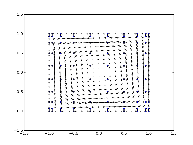
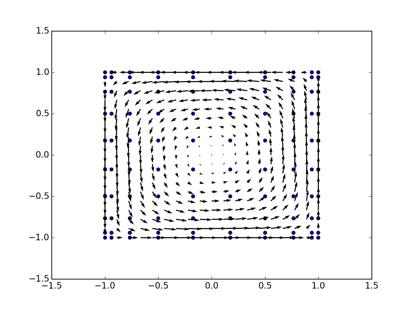
Figure 9
Plot for the solution of \((\star\mathbf{d}\star\mathbf{d}+\mathbf{d}\star\mathbf{d}\star)f\!=\!0\) with the boundary conditions of \(\star f |_{\mathcal{B}} = 0\) (vector field is tangent to the boundary) and \(\star\mathbf{d}\star f |_{\mathcal{B}}\!=\!1\) (the curl at the boundary is equal to \(1\)). The domain is \([-1,1]^2\), discretized by a \(10\!\times\!10\) Chebyshev grid.
(Source code, png, hires.png, pdf)